How To Evaluate & Manage Safety Risks In Biopharma

Of the many risks intrinsic to the pharmaceutical industry, safety has the most immediate significant impact. Safety risks can be described and modelled as cause-and-effect relationships using system risk structures (SRSs).¹ All risks are initiated by a cause that passes through a connecting mechanism, described as a system, to produce an effect. A specific risk must be defined and structured using all three elements — cause, system, and effect. The purpose of this article is to structure a broad range of risks beginning with a defined danger or threat so they can be effectively understood and then managed.

Safety belongs to a family of risks where the analysis of a primary risk begins with identifying an obvious primary threat (danger) that might pass through one or more primary systems to result in a primary consequence (harm). However, the probability of the danger resulting in harm may also depend on one or more secondary risk factors that impact the primary risk system’s ability to control the danger to prevent harm.

This article describes how a straightforward cause and effect model can be used to evaluate and manage safety risks. While all models are approximations and thus partially wrong, the portion that describes the risk’s structure can be useful in understanding how a danger results in harm. While safety risks are most frequently viewed in terms of preventing harm to an individual or a group of people, the same principles apply to preventing damage to equipment, business enterprises, or any subject from a well-defined threat or danger.

Risks are currently viewed and described by most risk practitioners, including the pharmaceutical industry, as bad events.^2,3,4 But effectively understanding a risk requires a more complete definition. Risk events do not occur spontaneously. All risk events are caused by a prior risk event. As shown in Figure 1, a primary risk is an input causal event (a threat) connected to the output effect event (a consequence) by a mechanism described as a control system. However, the system’s mechanism may be impacted by additional secondary risks that can also be described as a cause–system–effect relationship. A primary or simple risk is a linear sequence of the risk’s initiating threat, a connecting system mechanism, and the risk’s consequence. The connecting mechanism can be a sequence of systems. A complex risk is a network where the risk’s control system’s mechanism is significantly impacted by one or more secondary risk events.

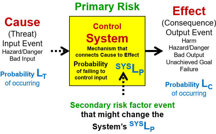
Figure 1: Definition of a risk – A primary risk is a possible cause that might pass through a system to result in an effect. For a simple risk, the probability of the effect L_C is the mathematical product of the probability of the cause L_T occurring and the probability ^SYSL_P that the threat will pass through the system, thus L_C = ^SYSL_P * L_T. The effect will not occur if the cause does not occur. For a complex risk, a secondary risk factor event might impact the probability of the primary risk’s ^SYSL_P significantly impacting the probability of the primary risk occurring should the threat occur.

All risk events have two attributes – severity and probability of occurrence. Severity can be easily described and rated from 0 to 7+ using Table A1 in the appendix. Table A1 covers seven orders of magnitude with an objective and subjective scale S_X, and a logarithmic rating value S_X^ calculated as the Log₁₀S_X of the objective scale. S_X^ provides a concise scale for describing the significance of any risk event ranging from 0 – no impact – to 7+ – catastrophic. The severity of the risk is defined as part of the risk’s definition. Different levels of severity are essentially different risks that have different probabilities of occurrence. The severity of risks is usually obvious or analyzed assuming a worst-case rating.

However, while risks are identified and initially prioritized by their severity, they are managed or controlled by their probability of occurrence. Unfortunately, probability of occurrence is far more challenging to estimate. The probability of any future event is always clouded by uncertainty. Some risk events, such as the role of a die, are mathematically definable, while others may have historical frequency data based on prior experience or experimentation. Estimating event probabilities other than well-defined fair games of chance involves complex uncertainties associated with the estimator’s level of knowledge and is subject to a variety of observer biases and prejudices. Thus, the challenge of managing any risk is objectively estimating the probability of a future event using the best available information, knowledge, and experience.

This article focuses on understanding and using a risk event’s probability of occurrence. A risk event’s probability or likelihood of occurrence can be described and rated using Table A2. Like the severity scale, the table covers seven orders of magnitude of probabilities L_X ranging from certain (100% or 1) to never (0% or 0). The likelihood table for a risk event X, either a causal threat or an effect consequence, includes both a subjective and objective scale, with the objective scale value (L_X) used to calculate a logarithmic rating value L_X^ as the logarithm of the objective scale. Values for ratings L_X^ range from 0 (certain) to ≤ -7 (essentially impossible). The ratings in Table A2 can be used to describe the probability of occurrence for any risk event. Estimating the probabilities of future events depends on the knowledge, expertise, and judgement of the evaluating individual or team making the estimate. If frequency data is available, it should be used.

Both Table A1 and A2 suggest that both severity and probability of occurrence only need to be estimated to an order of magnitude. Given the high subjectivity of both attributes, an order of magnitude is all that can be reasonably expected. The ultimate outcome of any risk analysis is to either accept the risk or make changes in the control system mechanisms to decrease the estimated probability of the risk consequence event occurring by one or more orders of magnitude to an acceptable level. Order of magnitude estimates for both attributes is sufficient to achieve eventual acceptance.

To quickly describe the significance of a risk event X for acceptance or remediation, the severity rating S_X^ (Table A1) and likelihood of occurrence rating L_X^ (Table A2) can be added together to provide an adjusted risk likelihood (ARL).⁵ An ARL value of zero (i.e., a 10% chance of losing $10 or a one in a million chance of losing a million dollars) appears to be a neutral point for accepting or rejecting many risks. Positive ARL values describe bad or difficult to accept risks while negative numbers describe more acceptable risks. Subjective consideration of the ARL in the context of the risk’s severity S_X^ provides a basis for reaching a consensus on risk acceptance decisions.

With a risk defined as one or more causal relationships and a risk event effectively described using a severity S_X^ and a likelihood L_X^ ratings, safety risks can be structured for analysis and management.

Simplified Model For Describing Safety Risks

Most safety risks can be modelled or described by the following three risk events separated by two control systems shown in Figure 2.

• Danger – a threat with a probability of occurrence L_D to the danger control system (DCS), usually from energy sources including chemical, gravitational, thermal, biological, kinetic, nuclear, and pressure.⁷ In many cases the danger is assumed to be certain with L_D = 100% (L_D^ = 0), as shown in Table A2. In some cases, the likelihood of the danger, such as an earthquake, may be lower.
• Hazard – a consequence output of the DCS that is a threat input to the hazard control system (HCS) of the probability L_H that could pass through the HCS to result in harm. If the danger is not controlled by the DCS, then the hazard must be controlled by the HCS.
• Harm – the risk consequence with a probability of occurrence of L_C resulting from a danger passing through both the DCS and HCS.

The primary risk is thus defined by the three events linked by the DCS and HCS. The control systems are the key to controlling the probability of a harmful event. The systems are modelled by the probability of the system failing to control the input threat to prevent the output consequence.

The probabilities or likelihoods of a threat successfully passing through a system are rated as shown in Table A3 in the appendix. The likelihood of the system shown in Figure 1 producing the output consequence L_C is the mathematical product of the likelihood of the threat occurring L_T and the likelihood ^SYSL_P that the system will propagate or fail to control the input. Thus L_C = ^SYSL_P * L_T. If the logarithmic ratings in Table A3 are used, then the output rating L_C^ is the sum of the input L_T^ and system ^SYSL_P^ likelihood ratings, thus L_C^ = ^SYSL_P^ + L_T^.

For the safety risk modeled by Figure 2, the two control systems work together in series to prevent the danger from resulting in the harm.

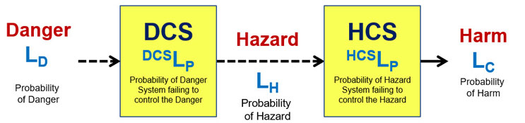
Figure 2: Danger Risk Structure model of a safety risk – The model shows the path from the danger to the harm. The model has the DCS composed of safety equipment that controls the danger from resulting in a hazard event. The HCS is human activity controlling the hazard to prevent the harm. If both control systems are effective, the likelihood of harm occurring, even for highly likely dangers, can be very low. For quick safety analysis, the DCS and HCS can be analyzed as a single system.

The DCS is protective equipment designed to have a probability of ^DCSL_P of controlling the danger event or situation to prevent a hazard. The DCS could range from simple personal protective equipment (PPE) to complex contamination control systems. As shown in Figure 2, the likelihood of the hazard being realized is L_H = L_D * ^DCSL_P. The HCS describes how people might observe potential hazards and modify their behavior or make other adjustments to decrease the likelihood of the hazard resulting in harm. The HCS reduces the probability of the possible hazard L_H from resulting in the harm L_C such that L_C = L_H * ^HCSL_P. The combined DCS and HCS have a cumulative probability of controlling the danger calculated as L_C = L_D * ^DCSL_P * ^HCSL_P. Thus, the danger is controlled by building control systems to make ^DCSL_P and ^HCSL_P as small as reasonably possible.

Depending on the specific safety risk, the primary risk can be described by only one of the two control systems. In some cases, ^DCSL_P >> ^HCSL_P places the burden of control on the HCS, requiring human observation and actions as the primary method of preventing harm. However, in other risks, ^DCSL_P << ^HCSL_P places the burden of controlling the danger on physical and mechanical systems, with little burden placed on human observation and actions because the likelihood of the hazard is minimal.

The key to analyzing any safety risk is to estimate the likelihood of the input danger L_D and the DCS and HCS likelihoods ^DCSL_P and ^HCSL_P. Evaluating the two ^SYSL_Ps must be done subjectively based on an evaluation and understanding of the mechanism of how the control systems were designed, constructed, and operated to minimize the likelihood of the input threats resulting in the output consequences.

However, both the DCS and HCS may be subject to important secondary risk events that must be identified and understood. The secondary risk events, should they occur, might significantly change ^DCSL_P or ^HCSL_P, thus the two likelihoods become essentially ranges with a focus on examining their worst-case values for properly evaluating the primary risk. In some cases, controlling the secondary risk events is vital to controlling the primary risk. If the system has a history, then frequency data may be available, but most often, a subjective estimate must be made on how the system is expected to perform, including the secondary risk factors.

Modeling Complex Safety Risks

Taking the simple primary risk structure shown in Figure 2 and adding secondary risk factors is shown in Figure 3. While a simple risk is a sequence, a complex risk occurs when a control system has both a primary threat and secondary threats, resulting in a network structure. While secondary risks cannot cause the primary risk consequence, they can significantly increase the likelihood of the primary risk threat, in this case the danger, passing through the primary control systems to result in the primary consequence (harm).

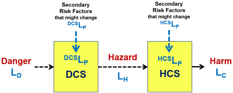
Figure 3: Danger Risk Structure model of a complex safety risk – A simple risk becomes a complex risk when the performance of the primary risk system (^SYSL_P) can be significantly impacted by secondary risk events (threats).

If the secondary risks are relatively obvious, then they can be included in the initial analysis of ^DCSL_P and ^HCSL_P. However, if the secondary risk factors are significant, they may need to be controlled. Thus, it may be appropriate to analyze the secondary risk factors in more detail as a complete cause-system-effect relationship to fully understand their potential impact on the primary safety systems and, when necessary and appropriate, introduce additional secondary risk control systems.

Modeling Secondary Risk Factors To A Primary Risk

Using the fundamental definition of a risk shown in Figure 1, secondary risks can be defined as prior threats that might pass through a threat control system (TCS) to result in a secondary risk event to a primary system. In the case of secondary risk factors, the threat’s consequence is a significant change by one or more orders of magnitude in a primary control system’s likelihood ^SYSL_P of propagating the primary threat input. A complex risk structure for a safety risk is shown in Figure 4.

Figure 4: Alternative SRS for describing a complex safety risk – The landscape describes vertically a primary risk of the danger producing harm and one or more secondary risk events impacting the performance of the primary control systems. Secondary risk events that significantly increase either ^DCSL_P or ^HCSL_P may require either changing the DCS or HCS to reduce the impact of the secondary threat or building TCSs that significantly reduce the probabilities of the secondary threats occurring to the primary control systems.

The landscape shown in Figure 4 introduces an approach for controlling important secondary threat events. The impact on the primary control systems results when secondary risks might increase by at least an order of magnitude a primary system’s probability of failure (^DCSL_P or ^HCSL_P), significantly increasing the chances of the primary risk occurring.

For a detailed risk analysis, the ^DCSL_P and ^HCSL_P might be viewed as ranges based on the probability of occurrence of the secondary risk events. In some cases, occurrence of the secondary risk events can completely compromise the ability of a control system to function, ^SYSL_P = 100%, requiring additional control systems to be added to better control the secondary threat.

While methods exist for rigorously solving the risk network structure describing both the primary and secondary risks, they are very difficult and far beyond the scope of this article. These methods include probabilistic graphs, Bayesian networks, or acyclic direct graphs.^7,8,9 Such advanced mathematical solutions may not be appropriate because of the high subjectivity and uncertainty of the information nor necessary to achieve order-of-magnitude estimates.

The approach used in this article is to decompose the primary and secondary risks and subjectively evaluate them separately and then collectively analyze them to understand and accept or remediate them as individual risks. While such an approach lacks mathematical rigor, the approach can be efficiently used by well-informed and experienced individuals and teams of experts to successfully manage a wide variety of risks.

As shown in Figure 4, secondary factors can be identified, modelled, and then individually evaluated as risks defined by Figure 1. If they are a significant threat to a primary control system, they can be remediated by developing a secondary threat control system that reduces the likelihood of the secondary threats occurring. In some cases, the control features for remediating the secondary threats can be placed within the primary control system’s design.

The following examples explain how simple and complex safety risks can be structured and evaluated in the context of possible secondary risk factors.

Example: Using Protective Gloves

The first example describes how a safety risk can be quickly viewed and analyzed. Figure 5 is one of several possible SRSs for analyzing the risk of using disposable gloves to prevent an operator’s hands from becoming contaminated when handling something that might be contaminated. The severity of the risk events (cause and effect) is determined by the nature of the contaminant and its possible impact on the subject.

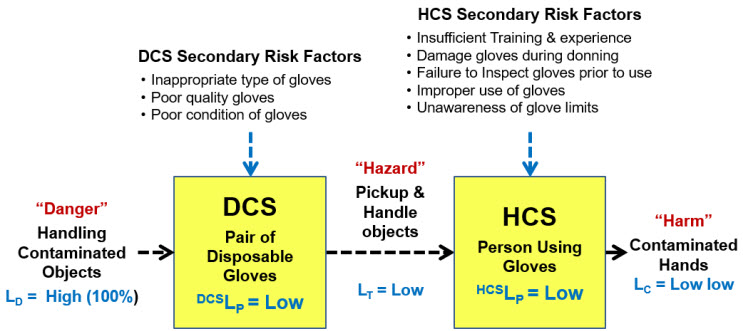
Figure 5: PPE Safety Risk – This SRS describes the risk of handling a contaminated object using gloves. The SRS is simple enough for an intuitive understanding of ^DCSL_P and ^HCSL_P to assess and manage both the primary and secondary risks.

In this example, the severity of the danger (the contaminant on the object) is assumed to be high and to be certain (L_D = 100%). If the gloves are used appropriately, they have a low probability (Low ^DCSL_P) of passing the contaminant to the user’s hands as a hazard. The secondary risk factors shown might impact the gloves’ ability to protect the subject by increasing ^DCSL_P and would be considered when estimating a value of ^DCSL_P. If the danger was particularly acute, secondary threat control systems can be implemented to minimize the likelihood of compromising the DCS’s performance. Also, if the likelihood of the contamination L_D is rare, the requirements for the DCS and HCS may be less rigorous.

The HCS also plays an important role in preventing harm by providing a low probability ^HCSL_P of the hands becoming contaminated by managing the interaction of the gloved hands and the contaminated object. Thus, using the estimated probabilities shown in Figure 5, the subject has a very low probability of harm. Of course, the analysis must consider a variety of secondary risk factors (inappropriate type of gloves, damaged glove, improper donning, etc.) in estimating the ^SYSL_P probabilities. Again, if the risk severity is potentially catastrophic, then additional secondary threat control systems can be implemented to reduce the likelihood of harm occurring from the primary risk.

The approach shown works for a wide variety of personal protective equipment such as face masks, personal behaviors such as social distancing to prevent transmitting airborne viruses, analyzing the risk of contaminating the surfaces of other objects, or other risks such as contaminating eyes, inhalation, etc.

Example: Handling Antibody-Drug Conjugates

A more complicated safety risk is summarized by the SRS shown in Figure 6. The handling of toxic compounds such as those used in antibody-drug conjugates (ADCs) poses a very serious risk to operators. The initial risk analysis might consider the two systems shown in Figure 6 to make an initial assessment of the primary risk, laying the foundation for a more detailed analysis that includes examining secondary risks and building the appropriate danger, hazard, and secondary threat control systems.

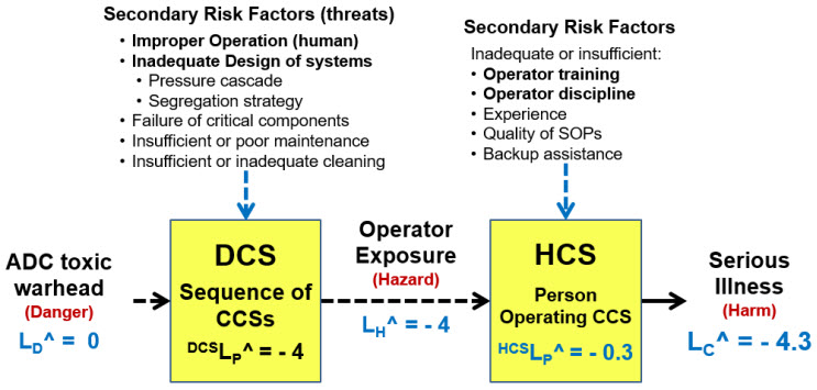
Figure 6: ADC safety risk – This is one possible SRS for managing safety risks for highly toxic warhead compounds required for making ADCs. Note that likelihood ratings are used instead of probabilities. The severity and probability guesses shown are for illustration purposes.

In this example, the likelihoods are described using the logarithmic scales shown in Figures A2 and A3. The danger likelihood is rated certain (L_C^ = 0). The team reaches a consensus that the DCS ^DCSL_P^ has a rating of -4 (0.01%) and the HCS a rating ^HCSL_P^ of -0.3 (50%) Thus, in the event of the hazard occurring, the HCS has only a 50% probability of preventing the harm. The two primary control systems have a combined ^SYSL_P^ of -4.3 (0.005%).

If the severity of the possible illness is S_C^ = >6 (Table A1), then the ARL for the risk is positive, making the DCS and HCS as described difficult to accept. If the risk is not acceptable, then the DCS and HCS can be improved to reduce the respective ^SYSL_P^s as evaluated by a team of experts to reduce L_C several orders of magnitude to reduce the ARL below zero. The DCS and HCS can be improved by building and evaluating SRSs for the important secondary risks that might compromise the control systems’ performance.

Each of the systems, especially the sequence of containment systems, might be expanded to fully understand how the danger of the toxic warhead to the operating personnel might be controlled to prevent harm. The expansion of the protection systems might include multiple threat paths (contact, inhalation) or multiple operational steps (setup, manufacturing, cleaning, changeout), requiring several SRSs be developed and evaluated. In some cases, probability estimates by experts may be confirmed or experimentally tested using challenge testing or frequency analysis of system steps and their performance mechanisms.

Most risks can be structured in several different ways depending on the experience and knowledge of the individual or team evaluating the risk. In many cases, sufficient knowledge and experience are available to reasonably estimate both the severity and likelihood of the threat events and the performance probabilities of the systems. However, additional information and experimental data should be collected to assure the probability estimates are the appropriate order of magnitude for the risk being evaluated.

Managing Safety Risks

The primary goal of this article is to present a simple approach for understanding safety risks. While the nomenclature may look complicated, the basic concept of using a causal definition for structuring the flow of threats and estimating probabilities to understand both simple and complex risks is relatively straightforward. By intuitively understanding how risks can be structured to describe the flow of risk events using simple thought experiments, individuals and teams can better assess situations to identify and accept or mitigate potential safety risks.

While risks are identified by their severity, they are managed by identifying, understanding, and, when necessary, manipulating their likelihood of occurrence. Understanding a risk is initiated by a thought experiment to identify how likely threats flow through systems to result in consequences of concern. By intuitively understanding the likelihood of the threat occurring and the likelihood of the systems controlling the threat in the context of secondary risk factors, an order of magnitude estimate of likelihood of harm can be guesstimated. Should the initial likelihood estimate be unacceptable in the context of the risk event’s severity, the primary control systems can be improved or additional systems added for controlling secondary risks, thus reducing the likelihood of the harm event occurring. Of course, an alternative approach of avoiding or removing the danger altogether, if possible, can also be explored.

References

1. Witcher, M., Principles and Concepts of System Risk Structures for Understanding and Managing Risks, Bioprocess Online, Dec. 6, 2021. https://www.bioprocessonline.com/doc/principles-and-concepts-of-system-risk-structures-for-understanding-managing-risks-0001
2. ISO 31000:2018 – Risk Management – International Organization for Standardization.
3. Hubbard, D. The Failure of Risk Management, Wiley, 2009.
4. FDA (CDER/CBER) – Guidance for industry: ICH Q9 quality risk management. June 2006. ICH.
5. Witcher, M., Rating Risk Events: Why Adjusted Risk Likelihood (ARL) Should Replace Risk Priority Number (RPN), Process Online, April 7, 2021 https://www.bioprocessonline.com/doc/rating-risk-events-why-we-should-replace-the-risk-priority-number-rpn-with-the-adjusted-risk-likelihood-arl-0001
6. Ericson, C.A., Hazard Analysis Techniques for System Safety, 2^nd Edition, Wiley & Sons. 2016.
7. Fenton, N. and M. Neil, Risk Assessment and Decision Analysis with Bayesian Networks, 2^nd edition, CRC Press, 2019.
8. Kjaerulff, U. and A. Madsen, Bayesian Networks and Influence Diagrams: A Guide to Construction and Analysis, 2^nd edition, Springer, 2013.
9. Sucar, L., Probabilistic Graphical Models – Principles and Applications, Springer, 2015.

Appendix – SRS Rating Scales

System risk structures (SRSs) require three simple scales that provide straightforward ratings for describing and managing risks. The logarithmic scales span the entire useful ranges and can provide simple rating values for describing and communicating a risk’s basic attributes. The first two tables describe a risk event’s attributes of severity of impact (Table A1) and probability (likelihood) of occurrence (Table A2). The third scale (Table A3) rates the likelihood that a system will fail to prevent an input threat such as a danger or hazard event from resulting in the output risk consequence event.

Table A1: A logarithmic scale of a risk’s impact severity from no impact (zero) to catastrophic (7+). A risk’s severity is described by the rating S_X^. A subjective scale is also provided.

Table A2: Scale for describing the probability of the risk events occurrence. The scale provides a rating L_X^ calculated as the logarithm of the probability. A rating of 0 represents certainty (100%). A rating of -7 represents a probability approaching zero (impossible).

Table A3: Scale that describes the likelihood, expressed as a probability, of system SYS not controlling the threat, thus producing the risk consequence. The scale produces a rating as the log of the probability that the input event will pass through the system to result in the output or outcome. If ^SYSL_P^ is equal to zero (certain), the system cannot control the threat. If ^SYSL_X^ equals -7, then the system is essentially a barrier that will prevent the input from producing the output.

About The Author:

Mark F. Witcher, Ph.D., has over 35 years of experience in biopharmaceuticals. He currently consults with a few select companies. Previously, he worked for several engineering companies on feasibility and conceptual design studies for advanced biopharmaceutical manufacturing facilities. Witcher was an independent consultant in the biopharmaceutical industry for 15 years on operational issues related to: product and process development, strategic business development, clinical and commercial manufacturing, tech transfer, and facility design. He also taught courses on process validation for ISPE. He was previously the SVP of manufacturing operations for Covance Biotechnology Services, where he was responsible for the design, construction, start-up, and operation of their $50-million contract manufacturing facility. Prior to joining Covance, Witcher was VP of manufacturing at Amgen. You can reach him at witchermf@aol.com or on LinkedIn (linkedin.com/in/mark-witcher).